Principal components analysis

Principal components analysis (PCA) is useful for data exploration and dimensionality reduction. In this post, we will see that (1) PCA is just an application of SVD, (2) PCs define an orthogonal coordinate system such that in this system the data are uncorrelated, (3) PCs maximize the variance explained in the data, and (4) we can often use a small number of PCs to reconstruct (or approximate) a given set of data.

What are principal components (PCs)?

Suppose we have a data matrix X with dimensions m x n, where each row corresponds to a different data point and each column corresponds to a different attribute.  (For example, if we measured the height and weight of 1000 different people, then we could construct a data matrix with dimensions 1000 x 2.)  Furthermore, let's presume that the mean of each column has been subtracted off (why this is important will become clear later).  If we take the SVD of X, we obtain matrices U, S, and V such that X = U*S*V'.  The columns of V are mutually orthogonal unit-length vectors; these are the principal components (PCs) of X.

SVD on the data matrix or the covariance matrix

Instead of taking the SVD of X (the data matrix), we can take the SVD of X'*X (the covariance matrix).  This is because X'*X = (V*S'*U')*(U*S*V') = V*S.^2*V' (where S.^2 is a square matrix with the square of the diagonal entries of S along the diagonal).  So, if we take the SVD of X'*X, the resulting V matrix should be identical to that obtained when taking the SVD of X (except for potential sign flips of the columns).  A potential benefit of taking the SVD of the covariance matrix is reduced computational time.  For example, if m >> n, then X is a large matrix of size m x n whereas X'*X is a small matrix of size n x n.

PCA decorrelates data

One way to think about PCA is that it decorrelates the data matrix.  Prior to PCA, the columns of the data matrix may have some correlation with each other, i.e. the dot-product of any given pair of columns of X may be non-zero.  What PCA does is to provide a linear transformation of the data such that after the transformation, the columns of the data matrix are uncorrelated with one another.  The transformation is specifically given by multiplication with the matrix V.

What exactly does multiplication with V do?  V has dimensions n x n and contains the principal components (PCs) in the columns.  Given a point in n-dimensional space (i.e. a vector of dimensions 1 x n), if we multiply that point with V, what we are doing is projecting the point onto each of the PCs.  This yields the coordinates of the point with respect to the space defined by the PCs.  Since the PCs form an orthogonal basis, all we are really doing is rotating the space.

Now let's see what happens when we take the data matrix X and multiply it with V.  Since X = U*S*V', X*V = U*S*V'*V = U*S.  The result, U*S, has the property that the columns are uncorrelated with one another.  The reason is that the columns of U are already mutually orthgonal by way of the SVD; and since S is a diagonal matrix, multiplication with S simply rescales the columns of U, which does not change the condition of mutual orthogonality.

% Let's see an example.  Here we create 1000 points
% in two-dimensional space.
X = zeromean(randnmulti(1000,[],[1 .6; .6 1],[1 .5]),1);
[U,S,V] = svd(X,0);
figure; setfigurepos([100 100 500 250]);
subplot(1,2,1); hold on;
scatter(X(:,1),X(:,2),'r.');
axis equal;
h1 = drawarrow([0 0],V(:,1)','k-',[],10,'LineWidth',2);
h2 = drawarrow([0 0],V(:,2)','b-',[],10,'LineWidth',2);
legend([h1 h2],{'PC 1' 'PC 2'});
xlabel('Dimension 1');
ylabel('Dimension 2');
title('Data');
subplot(1,2,2); hold on;
X2 = X*V;
V2 = (V'*V)';
scatter(X2(:,1),X2(:,2),'r.');
axis equal;
h1 = drawarrow([0 0],V2(:,1)','k-',[],10,'LineWidth',2);
h2 = drawarrow([0 0],V2(:,2)','b-',[],10,'LineWidth',2);
legend([h1 h2],{'PC 1' 'PC 2'});
xlabel('Projection onto PC 1');
ylabel('Projection onto PC 2');
title('Data');



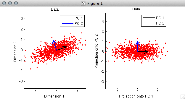
% In the first panel, we plot the data as red dots.  Notice
% that the two dimensions are moderately correlated with each other.
% By taking the SVD of the data, we obtain the PCs, and we plot
% the PCs as black and blue arrows.  Notice that the PCs are
% orthogonal to each other.  Also, notice that the first PC points
% in the direction along which the data tends to lie.
%
% In the second panel, we project the data onto the PCs and
% re-plot the data.  Notice that the only thing that has
% happened is that the space has been rotated.  In this new
% space, the data points are uncorrelated and the PCs are
% now aligned with the coordinate axes.

% Let's look at another example.  Whereas in the previous example
% we ensured that the columns of the data matrix were zero-mean,
% in this example, we will intentionally make the columns have
% non-zero means.
X = randnmulti(100,[1 -2],[1 .7; .7 1],[1 .5]);
% (now repeat the code above)



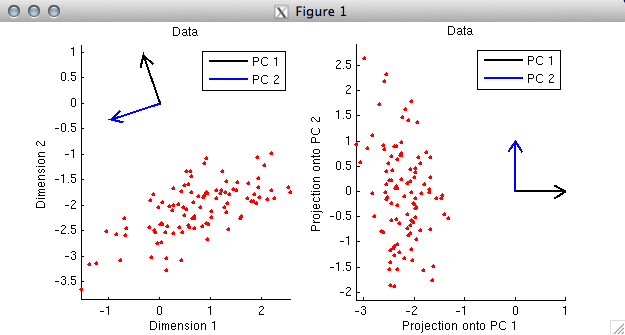
% In this example, the first PC again points in the direction along
% which the data tend to lie.  (Actually, strictly speaking, the
% first PC points in the opposite direction.  But there is a sign
% ambiguity in SVD --- the signs of corresponding columns of the U
% and V matrices can be flipped with no change to the overall math.
% So if we wanted to, we could simply flip the sign of the first PC (which
% corresponds to the first column of V) and also flip the sign of
% the first column of U.)  Notice that the first PC does not
% point in the direction of the elongation of the cloud of points;
% rather, the first PC points towards the middle of the cloud.
% The reason this happens is that the columns of the data matrix were not
% mean-subtracted (i.e. centered), and as it turns out, the primary effect
% in the data is displacement from the origin.
%
% (One consequence of neglecting to center each column is that the columns
% of the data matrix after projection onto the PCs may have some correlation
% with one another.  After projection onto the PCs, it is guaranteed only
% that the dot-product of the columns is zero.  Correlation (r) involves
% more than just a dot-product; it involves both mean-subtraction and
% unit-length-normalization before computing the dot product.  Thus, there
% is no guarantee that the columns are uncorrelated.  Indeed, in the
% previous example, the correlation after projection on the PCs is r=-0.23.)
%
% Whether or not to subtract off the mean of each data column before computing
% the SVD depends on the nature of the data --- it is up to you to decide.

PCs point towards maximal variance in the data

% Principal components have a particular ordering --- each principal
% component points in the direction of maximal variance that is
% orthogonal to each of the previous principal components.  In this
% way, each principal component accounts for the maximal possible
% amount of variance, ignoring the variance already accounted for
% by the previous principal components.  (With respect to explaining
% variance, it would be pointless for a given vector to be
% non-orthogonal to all previous ones; the extra descriptive
% power afforded by a vector lies only in the component of the
% vector that is orthogonal to the existing subspace.)

% Let's see an example.
X = zeromean(randnmulti(50,[],[1 .8; .8 1],[1 .5]),1);
figure; setfigurepos([100 100 500 250]);
subplot(1,2,1); hold on;
scatter(X(:,1),X(:,2),'r.');
axis equal;
xlabel('Dimension 1');
ylabel('Dimension 2');
title('Data');
subplot(1,2,2); hold on;
h = [];
for p=1:size(X,1)
  h(p) = plot([0 X(p,1)],[0 X(p,2)],'k-');
end
scatter(X(:,1),X(:,2),'r.');
scatter(0,0,'g.');
axis equal; ax = axis;
xlabel('Dimension 1');
ylabel('Dimension 2');
title('Variance of the data');



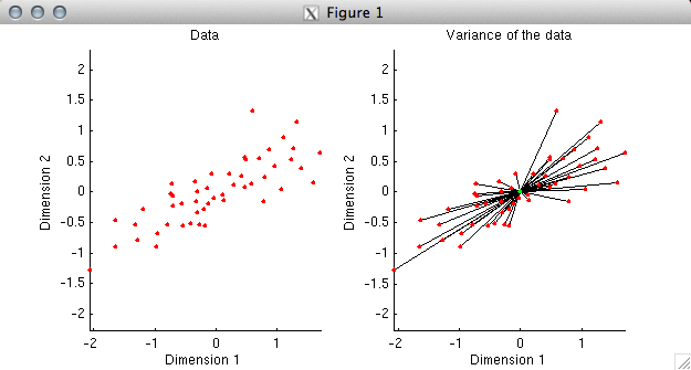
% In the first plot, we simply plot the data.  Before
% proceeding, we need to understand what it means to explain
% variance in data.  Variance (without worrying about
% mean-subtraction or the normalization term) is simply the
% sum of the squares of the values in a given set of data.
% Now, since the sum of the squares of the coordinates of a
% data point is the same as the square of the distance of the
% data point from the origin, we can think of variance as
% equivalent to squared distance.  To illustrate this, in the
% second plot we have drawn a black line between each data
% point and the origin.  The aggregate of all of the black lines
% can be thought of as representing the variance of the data.
% If we have a model that is attempting to fit the data, we
% can ask how close the model comes to the data points.
% The closer that the model is to the data, the more variance
% the model explains in the data.  Currently, without a model,
% our model fit is simply the origin, and we have 100% of the
% variance left to explain.
%
% What we would like to determine is the direction that accounts
% for maximal variance in the data.  That is, we are looking for
% a vector such that if we were to use that vector to fit the
% data points, the fitted points would be as close to the data
% as possible.
figure; setfigurepos([100 100 500 250]);
subplot(1,2,1); hold on;
direction = unitlength([.2 1]');
Xproj = X*direction*direction';
h = [];
for p=1:size(X,1)
  h(p) = plot([Xproj(p,1) X(p,1)],[Xproj(p,2) X(p,2)],'k-');
end
h0 = scatter(X(:,1),X(:,2),'r.');
h1 = scatter(Xproj(:,1),Xproj(:,2),'g.');
axis(ax);
xlabel('Dimension 1');
ylabel('Dimension 2');
title('Variance remaining for sub-optimal direction');
subplot(1,2,2); hold on;
[U,S,V] = svd(X,0);
direction = V(:,1);
Xproj = X*direction*direction';
h = [];
for p=1:size(X,1)
  h(p) = plot([Xproj(p,1) X(p,1)],[Xproj(p,2) X(p,2)],'k-');
end
h0 = scatter(X(:,1),X(:,2),'r.');
h1 = scatter(Xproj(:,1),Xproj(:,2),'g.');
axis(ax);
xlabel('Dimension 1');
ylabel('Dimension 2');
title('Variance remaining for optimal direction');



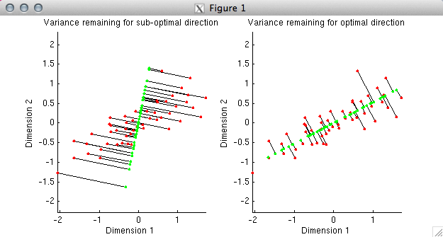
% In the first plot, we have deliberately chosen a sub-optimal
% direction (the direction points slightly to the right of vertical).
% Using the given direction, we have determined the best possible fit
% to each data point; the fitted points are shown in green.  The
% distance from the fitted points to the actual data points is
% indicated by black lines.  In the second plot, we have chosen the
% optimal direction, namely, the first principal component of the data.
% Notice that the total distance from the fitted points to the actual data
% points is much smaller in the second case than in the first.  This
% reflects the fact that the first principal component explains much
% more variance than the direction we chose in the first plot.
%
% The idea, then, is to repeat this process iteratively --- first,
% we determine the vector that approximates the data as best as
% possible, then we add in a second vector that improves the
% approximation as much as possible, and so on.

Singular values indicate variance explained

% A nice characteristic of PCA is that the PCs define
% an orthogonal coordinate system.  Because of this property,
% the incremental improvements with which the PCs approximate
% the data are exactly additive.
%
% (To see why, imagine you have a point that is located at (x,y,z).
% The squared distance to the origin is x^2+y^2+z^2.
% If we use the x-axis to approximate the point,
% the model fit is (x,0,0) and the remaining distance is
% y^2+z^2.  If we then use the y-axis to approximate the point,
% the model fit is (x,y,0) and the remaining distance is
% z^2.  Finally, if we use the z-axis to approximate the point,
% the model fit is (x,y,z) and there is zero remaining distance.
% Thus, due to the geometric properties of Euclidean space, all
% of the variance components add up exactly.)
%
% A little math can show that that the variance accounted
% for by individual principal components is given by the square of
% diagonal elements of the matrix S (which are also known as
% the singular values).
%
% The proportion of the total variance in a dataset that
% is accounted for by the first N PCs, where N ranges
% from 1 to the number of dimensions in the data can
% be calculated simply as
% cumsum(diag(S).^2) / sum(diag(S).^2) * 100.
% This sequence of percentages is useful when choosing
% a small number of PCs to summarize a dataset.
% We will see an example of this below.

Matrix reconstruction

% In data exploration, it is often useful to look at the big
% effects in the data.  A quick and dirty technique is to identify
% a small number of PCs that define a subspace within which
% most of the data resides.
temp = unitlength(rand(100,9),1);
X = randnmulti(11,rand(1,9),temp'*temp);
[U,S,V] = svd(X,0);
varex = cumsum(diag(S).^2) / sum(diag(S).^2) * 100;
Xapproximate = [];
for p=1:size(X,2)
  % this is a nice trick for using the first p principal
  % components to approximate the data matrix.  we leave it
  % to the reader to verify why this works.
  Xapproximate(:,:,p) = U(:,1:p)*S(1:p,1:p)*V(:,1:p)';
end
mn = min(X(:));
mx = max(X(:));
figure; setfigurepos([100 100 500 500]);
for p=1:size(X,2)
  subplot(3,3,p); hold on;
  imagesc(Xapproximate(:,:,p),[mn mx]);
  axis image; axis off;
  title(sprintf('PC %d, %.1f%% Variance',p,varex(p)));
end



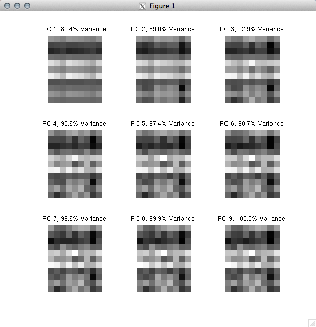
% What we have done here is to create a dataset (dimensions 11 x 9)
% and then use an increasing number of PCs to approximate the data.
% The full dataset corresponds to "PC 9" where we use all 9
% PCs to approximate the data.  Notice that using just 3 PCs
% allows us to account for 92.9% of the variance in the original data.
% 
% A useful next step might be to try and interpret the first 3 PCs
% and/or to visualize the data projected onto the first 3 PCs.
% If we gained an understanding of what is happening in the
% first 3 PCs of the data, it would probably be safe to deem that we
% have a good understanding of the data.