Geometric interpretation of linear regression

Linear regression can be given a nice intuitive geometric interpretation.

CODE

% Generate random data (just two data points)
y = 4+rand(2,1);

% Generate a regressor.
x = .5+rand(2,1);

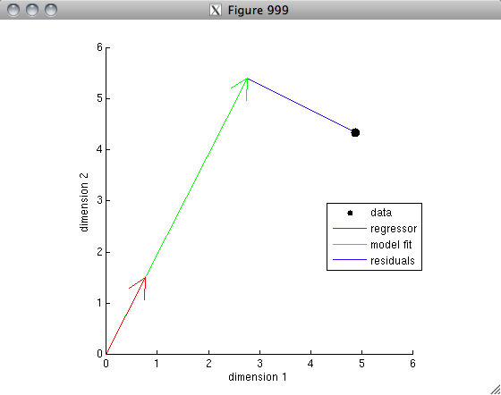
% Our model is simply that the data can be explained, to some extent,
% by a scale factor times the regressor, e.g. y = x*c + n, where c is
% a free parameter and n represents the residuals.  Normally, we
% want the best fit to the data, that is, we want the residuals to be
% as small as possible (in the sense that the sum of the squares of
% of the residuals is as small as possible).  This can be given
% a nice geometric interpretation: the data is just a single point
% in a two-dimensional space, the regressor is a vector in this space,
% and we are trying to scale the vector to get as close to the data
% point as possible.
figure(999); clf; hold on;
h1 = scatter(y(1),y(2),'ko','filled');
axis square; axis([0 6 0 6]);
h2 = drawarrow([0 0],x','r-');
xlabel('dimension 1');
ylabel('dimension 2');

% Let's estimate the weight on the regressor that minimizes the
% squared error with respect to the data.
c = inv(x'*x)*x'*y;

% Now let's plot the model fit.
modelfit = x*c;
h3 = drawarrow([0 0],modelfit','g-');
uistack(h3,'bottom');

% Calculate the residuals and show this pictorially.
residuals = y - modelfit;
h4 = drawarrow(modelfit',y','b-',[],0);
uistack(h4,'bottom');

% Put a legend up
legend([h1 h2(1) h3 h4],{'data' 'regressor' 'model fit' 'residuals'});



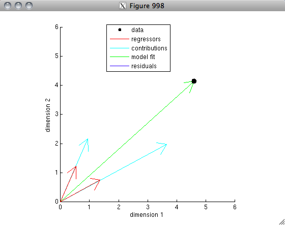
% OK. Now's let's do an example for the case of two regressors.
% One important difference is that the model is now a weighted sum
% of the two regressors and so there are two free parameters.
y = 4+rand(2,1);
x = .5+rand(2,2);
figure(998); clf; hold on;
h1 = scatter(y(1),y(2),'ko','filled');
axis square; axis([0 6 0 6]);
h2 = drawarrow([0 0; 0 0],x','r-');
xlabel('dimension 1');
ylabel('dimension 2');
c = inv(x'*x)*x'*y;
modelfit = x*c;
h3 = drawarrow([0 0],modelfit','g-');
uistack(h3,'bottom');
residuals = y - modelfit;
h4 = drawarrow(modelfit',y','b-',[],0);
uistack(h4,'bottom');

% Each regressor makes a contribution to the final model fit,
% so let's plot the individual contributions.
h3b = [];
for p=1:size(x,2)
  contribution = x(:,p)*c(p);
  h3b(p) = drawarrow([0 0],contribution','c-');
end
uistack(h3b,'bottom');

% Finally, put a legend up
legend([h1 h2(1) h3b(1) h3 h4],{'data' 'regressors' 'contributions' 'model fit' 'residuals'});



OBSERVATIONS

In the first example, notice that the model fit lies at a right angle (i.e. is orthogonal) to the residuals. This makes sense because the model fit is the point (on the line defined by the regressor) that is closest in a Euclidean sense to the data.

In the second example, the model fits the data perfectly because there are as many regressors as there are data points (and the regressors are not collinear).