CONCEPTS
In a previous post on correlation, we saw that the correlation between two sets of numbers is insensitive to the offset and gain of each set of numbers. Moreover, we saw that if you are using correlation as a means for measuring how well one set of numbers predicts another, then you are implicitly using a linear model with free parameters (an offset parameter and a gain parameter). This implicit usage of free parameters may be problematic --- two potential models may yield the same correlation even though one model gets the offset and gain completely wrong. What we would like is a metric that does not include these implicit parameters. A good choice for such a metric is the coefficient of determination (R^2), which is closely related to correlation.
Let <model> be a set of numbers that is a candidate match for another set of numbers, <data>. Then, R^2 is given by:
100 * (1 - sum((model-data).^2) / sum((data-mean(data)).^2))
There are two main components of this formula. The first component is the sum of the squares of the residuals (which are given by model-data). The second component is the sum of the squares of the deviation of the data points from their mean (this is the same as the variance of the data, up to a scale factor). So, intuitively, R^2 quantifies the size of the residuals relative to the size of the data and is expressed in terms of percentage. The metric is bounded at the top at 100% (i.e. zero residuals) and is unbounded at the bottom (i.e. there is no limit on the size of the residuals). This stands in contrast to the metric of r^2, which is bounded between -100% and 100%.
CODE
% Let's see an example of R^2 and r^2.
% Generate a sample dataset and a sample model.
data = 5 + randn(50,1);
model = .6*(data-5) + 4.5 + 0.3*randn(50,1);
% Now, calculate R^2 and r^2 and visualize.
R2 = calccod(model,data);
r2 = 100 * calccorrelation(model,data)^2;
figure(999); setfigurepos([100 100 600 220]); clf;
subplot(1,2,1); hold on;
h1 = plot(data,'k-');
h2 = plot(model,'r-');
axis([0 51 0 8]);
xlabel('Data point');
ylabel('Value');
legend([h1 h2],{'Data' 'Model'},'Location','South');
title(sprintf('R^2 = %.4g%%, r^2 = %.4g%%',R2,r2));
subplot(1,2,2); hold on;
h3 = scatter(model,data,'b.');
axis square; axis([0 8 0 8]); axissquarify; axis([0 8 0 8]);
xlabel('Model');
ylabel('Data');
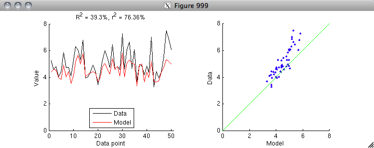
% Notice that r^2 is larger than R^2. The reason for this is that r^2
% implicitly includes offset and gain parameters. To see this clearly,
% let's first apply an explicit offset parameter to the model and
% re-run the "calculate and visualize" code above.
model = model - mean(model) + mean(data);
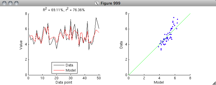
% Notice that by allowing the model to get the mean right, we have
% closed some of the gap between R^2 and r^2. There is one more
% step: let's apply an explicit gain parameter to the model and
% re-run the "calculate and visualize" code above. (To do this
% correctly, we have to estimate both the offset and gain
% simultaneously in a linear regression model.)
X = [model ones(size(model,1),1)];
h = inv(X'*X)*X'*data;
model = X*h;
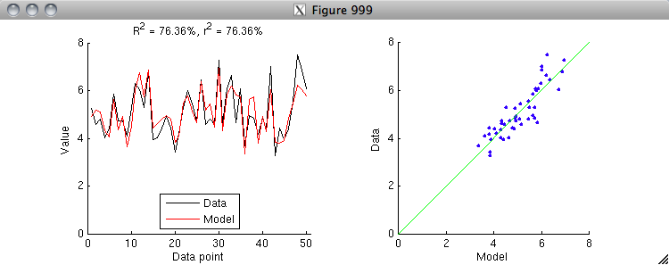
% Aha, the R^2 value is now the same as the r^2 value.
% Thus, we see that r^2 is simply a special case of R^2
% where we allow an offset and gain to be applied
% to the model to match the data. After applying
% the offset and gain, r^2 is equivalent to R^2.
% Note that because fitting an offset and gain will
% always reduce the residuals between the model and the data,
% r^2 will always be greater than or equal to R^2.
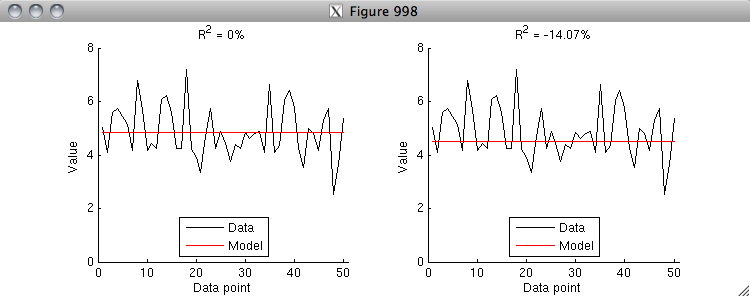
% In some cases, you might have a model that predicts the same
% value for all data points. Such cases are not a problem for
% R^2 --- the calculation proceeds in exactly the same way as usual.
% However, note that such cases are ill-defined for r^2, because
% the variance of the model is 0 and division by 0 is not defined.
% An R^2 value of 0% has a special meaning --- you achieve 0% R^2
% if your model predicts the mean of the data correctly and does
% nothing else. If your model gets the mean wrong, then you can
% quickly fall into negative R^2 values (i.e. your model is worse
% than a model that simply predicts the mean). Here is an example.
data = 5 + randn(50,1);
model = repmat(mean(data),[50 1]);
R2 = calccod(model,data);
figure(998); setfigurepos([100 100 600 220]); clf;
subplot(1,2,1); hold on;
h1 = plot(data,'k-');
h2 = plot(model,'r-');
axis([0 51 0 8]);
xlabel('Data point');
ylabel('Value');
legend([h1 h2],{'Data' 'Model'},'Location','South');
title(sprintf('R^2 = %.4g%%',R2));
subplot(1,2,2); hold on;
model = repmat(4.5,[50 1]);
R2 = calccod(model,data);
h1 = plot(data,'k-');
h2 = plot(model,'r-');
axis([0 51 0 8]);
xlabel('Data point');
ylabel('Value');
legend([h1 h2],{'Data' 'Model'},'Location','South');
title(sprintf('R^2 = %.4g%%',R2));
% Finally, note that R^2 is NOT symmetric (whereas r^2 is symmetric).
% The reason for this has to do with the gain issue. Let's see an example.
data = 5 + randn(50,1);
regressor = data + 4*randn(50,1);
X = [regressor ones(50,1)];
h = inv(X'*X)*X'*data;
model = X*h;
r2 = 100 * calccorrelation(model,data)^2;
figure(997); setfigurepos([100 100 600 220]); clf;
subplot(1,2,1); hold on;
R2 = calccod(model,data);
h1 = scatter(model,data,'b.');
axis square; axis([0 8 0 8]); axissquarify; axis([0 8 0 8]);
straightline(mean(data),'h','k-');
xlabel('Model');
ylabel('Data');
title(sprintf('R^2 of model predicting data = %.4g%%; r^2 = %.4g%%',R2,r2));
subplot(1,2,2); hold on;
R2 = calccod(data,model);
h2 = scatter(data,model,'b.');
axis square; axis([0 8 0 8]); axissquarify; axis([0 8 0 8]);
straightline(mean(data),'h','k-');
xlabel('Data');
ylabel('Model');
title(sprintf('R^2 of data predicting model = %.4g%%; r^2 = %.4g%%',R2,r2));
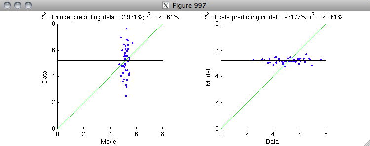
% On the left is the correct ordering where the model is attempting to
% predict the data. The variance in the data is represented by the scatter
% of the blue dots along the y-dimension. The green line is the model fit,
% and it does a modest job at explaining some of the variance along the
% y-dimension. It is useful to compare against the black line, which is the
% prediction of a baseline model that only and always predicts the mean of
% the data. On the right is the incorrect ordering where the data is
% attempting to predict the model. The variance in the model is represented
% by the scatter of the blue dots along the y-dimension. The green line is
% the model fit, and notice that it does a horrible job at explaining the
% variance along the y-dimension (and hence explains the very low R^2 value).
% The black line is much closer to the data points than the green line.
%
% Basically, what is happening is that the gain is correct in the case at
% the left but is incorrect in the case at the right. Because r^2
% normalizes out the gain, the r^2 value is the same in both cases.
% But because R^2 is sensitive to gain, it give very different results.
% To fix the case at the right, the gain on the quantity being used for
% prediction (the x-axis) needs to be greatly reduced so as to better
% match the quantity being predicted (the y-axis).
Thanks Kendrick,
ReplyDeleteGreat blog!
Nikola
Very impressive and informative blog.Thanks for such an useful information.
ReplyDeleteThanks for sharing it.www.youtube.com/watch?v=SrzMdoKPPaA
ReplyDeletegörüntülü show
ReplyDeleteücretlishow
Lİ12NF
https://titandijital.com.tr/
ReplyDeletekilis parça eşya taşıma
bursa parça eşya taşıma
ığdır parça eşya taşıma
bitlis parça eşya taşıma
4TR6PM
HGNHGMJHK
ReplyDeleteمكافحة حشرات
Cool and that i have a keen present: How To Renovate House Exterior zombie house renovation
ReplyDeleteشركة تنظيف بالاحساء hZX4w4axWm
ReplyDeleteشركة عزل اسطح بالقطيف JrvLmLUPvk
ReplyDelete